![]()
![]()
![]()
In Chapter 1, we explained how retrieval of similar cases relates to CBR, fuzzy logic, and weather prediction-CBR depends on retrieval of similar cases, fuzzy logic enables retrieval of similar cases, and the weather prediction technique of analog forecasting depends on retrieval of similar cases-and explained how case adaptation and case authoring are regarded as main challenges in CBR system development. In Chapter 2, we described how, to overcome the case adaptation and case authoring problems of CBR system development, three strategies have been proposed-knowledge acquisition, partial matching, and use of very large cases bases-and surveyed the literature to provide a basis for using the fuzzy k-nn technique to combine these strategies into one technique.
In this chapter, we describe the WIND-1 system. The system uses a fuzzy k-nn algorithm designed to emulate a weather forecasting expert applying the weather prediction technique of analog forecasting and, thereby, shows how fuzzy logic based methods enable a CBR system developer to impart the perceptiveness and case-discriminating ability of a domain expert to CBR. We describe the necessary details in as general terms as general as possible. Though the WIND-1 system is specifically designed for weather prediction, similar systems should be applicable to other kinds of analog prediction problems where large databases exist and perceptive experts are available to help to tune similarity-measuring fuzzy sets.
The WIND-1 system consists of two main parts:
· A large database of weather observations. The database is a weather archive of over 300,000 consecutive hourly weather observations.
· A fuzzy k-nn algorithm. The algorithm measures the similarity between temporal cases, past and present intervals of weather observations. The algorithm is tuned with the help of a domain expert, in our case, a weather forecaster experienced in noting similarities between cases.
Section 3.1 describes the database: an archive of airport weather observations. Section 3.2 describes our fuzzy k-nn algorithm which searches the database for analogs. Section 3.3 compares our fuzzy k-nn approach case-based reasoning with two previous approaches. In the next Chapter 4, we will present a set of experiments and results based upon the WIND-1 system.
3.1 Large database of airport weather observations
Airport weather observations (METAR's) are routinely made at all major airports on the every hour on the hour. Our database consists of a flat-file archive of 315,576 consecutive hourly weather observations from Halifax International Airport. 60 These observations are from the 36-year period from 1961 to 1996, inclusive. Based on the advice of a weather forecaster, we represent each hour with 12 selected attributes: 11 continuous attributes and 1 nominal attribute, precipitation, as shown in Figure 10.
Category |
Attribute |
Units |
temporal |
· date |
Julian date of year (wraps around) |
· hour |
hours offset from sunrise/sunset | |
cloud ceiling |
· cloud amount(s) |
tenths of cloud cover (for each layer) |
and visibility |
· cloud ceiling height |
height in metres of ³ 6/10ths cloud cover |
· visibility |
horizontal visibility in metres | |
wind |
· wind direction |
degrees from true north |
· wind speed |
knots | |
precipitation |
· precipitation type |
"nil", "rain", "snow", etc. |
· precipitation intensity |
"nil", "light", "moderate", "heavy" | |
spread and |
· dew point temperature |
degrees Celsius |
temperature |
· dry bulb temperature |
degrees Celsius |
pressure |
· pressure trend |
kiloPascal · hour -1 |
Figure 10. Twelve attributes of an airport weather observation (METAR).
The file size is 6 Megabytes. The file is in a standard, column-delimited ASCII format, hence no preprocessing is needed. Very few values are missing and most of the reports appear to be reliable (i.e., plausible), hence no additional quality control is applied to the file prior to its use.
This section explains how we built an expert-emulating, similarity-measuring fuzzy k-nn algorithm, or function. The similarity-measuring function, sim, is used to find k nearest neighbors. The function is given two cases, each identified by unique time indexes t1 and t2, and it returns a real number proportional to the degree of similarity of the two cases such that
0.0 < sim(t1, t2) £ 1.0
Because all weather cases are unique and because the value of sim is calculated to double precision, sim can identify exactly k nearest neighbors. There are no null search results and no ties.
The three steps to construct and use the algorithm are:
1. Configure similarity-measuring function.
2. Traverse case base to find k-nn.
3. Make prediction based on weighted median of k-nn.
The first step is performed only once and the second and third steps are performed every time weather prediction is made. All the algorithm design work is done in the first step. The steps are described in the following three subsections (3.2.1, 3.2.2, and 3.2.3).
3.2.1 Configure similarity-measuring function
To configure the function, an expert weather forecaster uses a fuzzy vocabulary to provide knowledge about how to perform case comparisons. A detailed sample questionnaire for knowledge acquisition is shown in Appendix A. The knowledge acquisition procedure is described in general terms in the following two subsections.
3.2.1.1 Expert specifies attributes to compare and the order in which they are to be compared
An expert suggests which attributes are important for matching. For the WIND-1 system, we selected the 12 attributes listed above in Figure 10.
An object is to summarily rule a case out of contention with the fewest possible number of tests. Hence, based on advice of the domain expert, tests most likely to discriminate are performed first. For instance, the expert suggests that the season attribute similarity be tested before the temperature attribute similarity. Winter cases are very unlike Summer cases, but a winter case and a summer case may both have temperatures of 10º Celsius. Therefore, date of the year is a better discriminator than temperature.
When cases are compared, their attributes are compared in the same order that they are listed in in Figure 10, namely: date of the year, hour of the day, cloud amount(s), cloud ceiling height, visibility, wind direction, wind speed, precipitation type, precipitation intensity, dew point temperature, dry bulb temperature, and pressure trend. When initial tests indicate great dissimilarity, subsequent tests are dispensed with.
3.2.1.2 Expert describes fuzzy relationships between attributes
This is the crucial step in system design. As the expert describes fuzzy relationships between attributes using fuzzy words, corresponding fuzzy sets are constructed to emulate expert case comparison. Appendix A shows a sample questionnaire for knowledge acquisition that a developer could ask a domain expert complete in order to obtain knowledge of how to evaluate degree of similarity between various comparable attributes of cases. Thereby, the expert imparts their sense of discrimination via fuzzy words into fuzzy sets, and we acquire knowledge about how to compare three kinds of attributes: continuous numbers, absolute numbers (i.e., magnitude), and nominal attributes (e.g., snow and rain) . And we acquire knowledge about how to weight recency, or in other words, how to forget older dissimilarities. This acquired knowledge is represented below in four functions -
m
c,
m
a,
m
n,
m
f-in the following four sections in Figure 11, Figure 12, Figure 13, and Figure 14 (b).
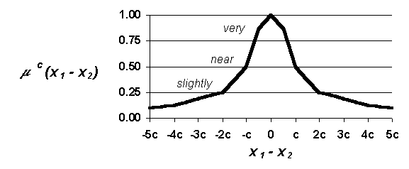
Continuous-number attributes
For each continuous attribute, xi, the expert specifies a value of ci which is the threshold for considering two such attributes to be near each other. A fuzzy set is constructed accordingly as shown in Figure 11. Figure 11. Fuzzy set for comparing continuous-number attributes. Similarity-measuring function emulates how the expert evaluates the degree to which continuous attributes are near each other. The expert specifies a value of c corresponding near such that
m(x1 - x2)
³
0.50
Û
"x1 is near x2".
Tails taper off asymptotically towards 0.0, such that
m(x) > 0.0, which prevents null results from searches.
Comparing two homogeneous, continuous attributes with a fuzzy set, as shown in Figure 11, is a basic application of fuzzy sets. Multiple attributes of cases can be weighed collectively by aggregating the result of a set of such operations (e.g., taking the "max of the min"). Each fuzzy set enables the sim function to match based on individual attributes. As sets are added for multiple attributes, the sim function gains the ability to match more complicated cases.
Fuzzy sets such as the one shown in Figure 11 are used to compare the attributes of date of the year, hour of the day, wind direction, dew point temperature, dry bulb temperature, and pressure trend.
Date of the year and hour of the day are important temporal attributes because weather strongly correlates to seasonal and diurnal cycles. The closer these attributes of two cases are to each other, the more analogous the cases are. For example, two cases are considered near each other if they are within 30 Julian days of each other and their offsets from sunrise/sunset are within one hour of each other.
Absolute-number attributes
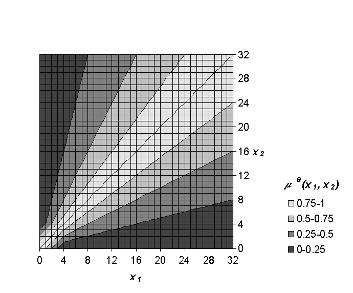
If attributes are limited to the zero-or-above range (e.g., absolute wind speed), then it is their relative magnitudes that are important for matching. Therefore, they are compared using a modified ratio operation, with special routines to handle for values near zero, as shown in Figure 12. Figure 12. Fuzzy decision surface for comparing absolute-number attributes. Fuzzy similarity-measuring surface measures how similar two absolute values are to each other. The above surface determines the similarity of two wind speeds, x1 and x2, where speed is measured in knots. Wind speed values above 32 are truncated to 32. The fuzzy decision surface shown in Figure 12 is used to compare the attribute of wind speed. Surfaces similar to the one shown in Figure 12 are used to compare the attributes of cloud amount(s), cloud ceiling height, and visibility.
Nominal attributes
To compare nominal attributes, such as precipitation type, a similarity measuring table (a symmetric matrix) is used of the form shown in Figure 13.
The table of fuzzy relationships shown in Figure 13 is used to compare the attribute of precipitation type. A table similar to that shown in Figure 13 is used to compare the attribute of precipitation intensity. Nil Drizzle Showers Rain Flurries Snow ... Nil 1.00 0.02 0.03 0.01 0.03 0.01 ... Drizzle 0.02 1.00 0.50 0.50 0.10 0.05 ... Showers 0.03 0.50 1.00 0.75 0.10 0.10 ... Rain 0.01 0.50 0.75 1.00 0.10 0.25 ... Flurries 0.03 0.10 0.10 0.10 1.00 0.75 ... Snow 0.01 0.05 0.10 0.25 0.75 1.00 ... ... ... ... ... ... ... ... ... mn(type1, type2) Figure 13. Fuzzy relationships between nominal attributes. Similarity-measuring table measures how similar two nominal attributes are to each other. Forget older attributes
The similarity of two cases is determined according to their newest and their most dissimilar attributes. 61 The older attributes are in compared cases-that is, the farther back in time they are from their respective time-zeroes- the less weight is accorded to their dissimilarity. In effect, this is the same as forgetting older attributes in comparing cases. Such a forgetting function is shown in Figure 14 (b). After two comparable attributes of two cases are compared to yield a similarity value,
m´,
the value of sim = max {m´,
So, with reference to Figure 14 (b), we see that 3-hour-old attributes can never imply sim < 0.6, whereas time-zero attributes or auxiliary predictors (with t > 0), can imply sim
@
0.0.
The more recent an attribute is, the more important it is for matching. Likewise, any auxiliary predictors, such as NWP, are important for matching. Each case has a temporal span of 24 hours composed of three parts: 12 recent past hours, 1 time-zero hour, and 12 future hours. (These three parts of a case are illustrated ahead in Figure 16, page 87.) The contributions to similarity measurement of cases, from corresponding hours of cases, are weighted to maximize the contribution of recent hours and to maximize the contribution of any available foreknowledge (e.g., prevision guidance from NWP), as shown in Figure 14. (a) Recency weighting function. The newer attributes in compared cases are, the more their similarity is weighted. Greatest weight is given to recent attributes and future attributes, such as auxiliary predictors from NWP. (b) Forgetting function. This function is the complement of the above recency weighting function, Figure 14 (a). The newer attributes in compared cases are, the stricter their similarity comparison. Corresponding hour-to-hour comparisons are "maxed" with the forgetting function. Thus, for example, comparison of attributes 3 hours prior to time-zero will result in similarity
m
³
0.6; whereas, comparison of attributes measured at time-zero, or predicted by other means for after time-zero, may result in similarity
m
= 0.0. Thus, the function emulates the forgetting of less relevant older attributes in case-to case comparison. Figure 14. Fuzzy weighting for recency of attributes. 3.2.2 Traverse case base to find k-nn
After sim has been configured as explained above, it can be used to make weather predictions provided with a database of weather cases, a present incomplete weather case, and whatever foresight-offering guidance is available. Appendix B shows a worked-out, specific example of the procedure for making a prediction based on the fuzzy k-nn. The rest of this subsection illustrates the procedure generally.
First, for each hour of two cases being compared, the overall degree of similarity of their attributes is computed as the minimum value of
m
for the compared attributes. mhour-to-hour(t) = min{mc1, ... , m ai, ... , mnm } for t = t0-12 ... t0 Second, the overall degree of the similarity of two cases is computed as the minimum value of all the hours' values of
m
where each hour's value of
m
is tempered by the "forgetting function." mcase-to-case(t0) = min{max{
m
hour-to-hour(t0-12),
m
f(-12)}, ... , max{
m
hour-to-hour(t0),
m
f(0)}} The database of cases is represented conceptually in Figure 15. Each block represents an observation taken at one instant in time. Observations are taken at regular intervals. So, the series of blocks represents the time series. a1(1)
a2(1)
:
am(1) a1(2)
a2(2)
:
am(2) ... a1(n)
a2(n)
:
am(n) Figure 15. Structure of cases (i.e., weather observations). m attributes per observation, n observations. Observation is synonymous with tuple.
The parts of a temporal case are shown in Figure 16. A temporal case is a short segment of a long record of a multidimensional, real-world process-in our case, weather observations. Past cases in the database are complete temporal cases. The present case is an "incomplete temporal case"-it's missing the "future" part.
¾¾¾
time
¾¾®
recent past time zero future a(t-12) a(t-11) ... a(t) ... a(t+12) Figure 16. Temporal case. A series of weather observations centered on time t. Thus t is the specific case index. Series spans from 12 hours before to 12 hours after time t.
The time series of past cases is traversed and temporal cases are measured for degree of similarity with the present case using sim as shown in Figure 17.
Past Present Levels of tests a1(i-12)
a1(j-12)
: è : è case-to-case a1(i+12)
a1(j+12)
(series-to-series) a1(i)
è a1(j)
è tuple-to-tuple
a1(i) ® a1(j) ® attribute-to-attribute Figure 17. Temporal cases are compared in nested operations at three levels. Specific case indexes are i and j, the "time-zeros" of the cases being compared. The "®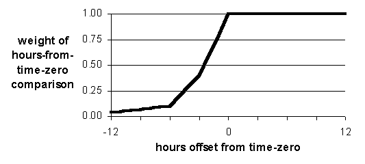

case
case
in sim function
:
am(i-12)
:
am(j-12)
:
am(i+12)
:
am(j+12)
:
am(i)
:
am(j)
(vector-to-vector)
The overall similarity of two temporal cases is equal to the lowest similarity of any comparable elements (i.e., equal to the lowest attribute-to-attribute similarity). The sim function performs tests progressively, following the efficiently discriminating sequence advised by the expert (subsection 3.2.1.1). The similarity measuring operation is halted if the similarity falls below the a-level (i.e., the current minimum threshold to join the analog set). As better and better analogs are collected during the traversal, the a- level rises accordingly. As the a-level rises, the case-to-case comparison can be aborted after fewer and fewer attribute-to-attribute comparisons. Thus, although the above 3-level-deep case comparison algorithm is potentially of Order(n3) complexity, in practice we expect it to be much closer to Order(n) complexity.
The analogs are collected and a is recorded in a linked list data structure as shown in Figure 18.
|
|||||
® |
|
||||
¯ |
|||||
|
|||||
Contraints |
¯ |
||||
0 £ list_length £ k |
: |
||||
max_sim = a |
¯ |
||||
min_sim > 0.0 |
|
||||
^ |
|||||
Figure 18. Linked list of k-nn, or weather analogs. The similarity of each case is represented by sim[i]. By design,
0.0 < sim[i]
£
1.0. The least similar member in the set has overall similarity equal to sim[k], thus a-level = sim[k]. list_length is the number of cases in the list.
max_sim and min_sim describe the similarity values of the most
similar and least similar cases in the list respectively.
index[i] identifies the time of the temporal case.
3.2.3 Make prediction based on weighted median of k-nn
The predictands are cloud ceiling and visibility. Predictions are made by weighted median of the k most analogous cases, the k-nn. Each case is weighted according to its similarity to the present case: 0.0 < sim[i] £ 1.0.
A worked-out example of how the fuzzy k-nn algorithm measures the similarity of two temporal cases with a present case and makes predictions based on the fuzzy k-nn is shown in Appendix B.
3.3 Comparison to previous approaches
This section compares our fuzzy k-nn algorithm with a classic fuzzy nearest prototype algorithm and with a classic model of CBR.
3.3.1 Fuzzy nearest prototype algorithm
Compare our fuzzy nearest prototype algorithm in Figure 19 and Figure 20 with that of Keller et al. (1985), shown in Figure 8 (page 60).
Let W = {A1, A2, ..., An} be the set of n past cases representing n potential analogs.
// x is the present case
main(x)
{
a = 0.0
list_lenth = 0
// traverse past case base of n cases searching for analogs
for i = 1 to n
{
// test all past cases for admissibility into the k-nn set
// a is the admission threshold
// if similarity of new case > a
// then new case is saved and a rises accordingly
if (sim(Ai, x) > a)
{
a = sim(Ai, x)
// Update the linked list of k-nn, shown in Figure 18 on page 88
insert_to_ordered_k-nn_list(Ai)
// limit list length to k
list_length = list_length + 1
if list_length > k
{
remove_from_ordered_k-nn_list_least_similar_member()
list_length = list_length - 1
}
}
}
return(weighted median of k-nn)
}
where sim(Ai, x) is represented by the function shown in Figure 20.
Figure 19. Cyclic algorithm for WIND-1 in pseudocode. Nearest prototype algorithm centered on the present case and with a-level progressively rising as case base is traversed and better analogs accumulate in ordered k-nn list. This algorithm contrasts with that of Keller et al. (1985), which is shown in Figure 8 on page 60.
double sim(Ai, x)
{
// result = 1.0 implies similar, result = 0.0 implies dissimilar
result = 1.0
// traverse series from most recent tuple to least recent tuple
// h is the number of hours in a temporal case
for h = tuples_in_series down to 1)
{
for (m = 1 to attributes_in_tuple)
{
// mm is an attribute-specific fuzzy comparison operation,
// i.e, ma, m c, and m n as shown Figure 11, Figure 12, and Figure 13
// on pages 81-83
result = mm(Ai[h, m], x[h, m])
// Reduce weight of old attributes in case
// result approaches 1.0 for non-recent attributes
// In effect, calculate maximum of result with
// of fuzzy set shown in Figure 14 (b) on page 85.
weight_for_recency(result)
if (result < a)
return (0.0)
}
}
Figure 20. Similarity-measuring function: sim.
Our algorithm differs from that of Keller et al. (1985) mainly in the following way: Rather than calculating the distance from the new case to every selected prototypical case and then, accordingly, calculating the degrees of membership of the new case in all the prototypical categories as (Keller et al. 1985) does, our algorithm calculates the degrees of similarity between the present case and its k nearest neighbors. Only the k instances of Ai that are nearest to the present case are assigned values for degree of similarity to the present case. Our approach is, in a sense, a reversal of that of Keller et al.: Rather than calculating the degrees of membership of the present case in selected categories, which are based on prototypes, we calculate the degrees of membership of past cases in the one-off "category" that is based on the present case.
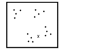
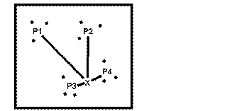
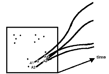
As the case base is traversed, and each prospective analog Ai is subjected to a series of similarity tests, cases are either summarily ruled out of contention or finally ruled into the k-nn set. As the case base is traversed, and better and better analogs are collected, the a- level rises accordingly. This strategy enables computational savings. Because we are only interested in identifying exactly k nearest neighbors, most of the past cases can be summarily ruled out of contention. Rather than fully calculating the similarities between a new case and all predefined prototypes, as illustrated in Figure 21 (b), it predicts the outcome of the new case based on a few nearest neighbors, as illustrated in Figure 21 (c).
|
(a) Points represent past cases.
(b) New case X is classified according to distance from selected prototypes, P1-P4. |
(c) New case is predicted for based on outcome of nearest neighbors, A1-A4 (i.e., the "analog ensemble.") |
Figure 21. Classification based on prototypes contrasted with prediction based on nearest neighbors. (a) A number of fully-described points and one new partly-described point labelled as X. (b) Classification of a new case based on selected prototypes. (c) Prediction for a new case based on k nearest neighbors.
3.3.2 Classic case-based reasoning
Compare our case-based reasoning flowchart, shown in Figure 22, with that of Riesbeck and Schank (1989), shown in Figure 1 (page 4). The differences between classic CBR and fuzzy CBR are listed in Figure 23.
Inference Engine |
Knowledge Base |
Problem |
® |
Input |
||
¯ |
||||
Many |
® |
Retrieve |
¬ |
Fuzzy Matching |
Automatically |
¯ |
Function | ||
Recorded |
k-nn |
|||
Cases |
¯ |
|||
Adapt |
¬ |
Adaptation Rule: | ||
¯ |
Calculate Median of | |||
Solution |
¬ |
Median and |
k-nearest neighbors | |
Confidence |
¬ |
Spread |
Figure 22. Fuzzy case-based reasoning. This flowchart contrasts with that of Riesbeck and Schank (1989), which resembles the one shown in Figure 1 (page 4). The case authoring problem is avoided by using many automatically-recorded cases and a fuzzy matching function. The case adaptation problem is avoided by using many automatically-recorded cases (with supposed good analogs) and by simply calculating a median of k-nearest neighbors.
Classic CBR |
Fuzzy CBR |
· Uses abstract indexing rules to determine classes. |
· Describes cases with their numerical dimensions and nominal types. |
· Revises the case memory with tested solutions. |
· Uses a large case base of continuously accumulating actual cases. |
· Attempts to repair solutions in a potentially endless loop. |
· Bases solution on a weighted median of numerous similar cases and associates a confidence in the solution based on the spread of those cases. |
· Perform the series of operations: Proposed Solution ® Test ® Failure Description ® Explain ® Predictive Features ® Indexing Rules. |
· Obtains knowledge about predictive features through knowledge acquisition from domain expert who explains similarity with fuzzy words. |
Figure 23. Differences between classic CBR and fuzzy CBR.
60 Halifax International Airport is located in Nova Scotia, Canada at coordinates 44º 53' North 63º 30' West at an elevation of 145 meters above sea level. The airport is situated 30 kilometers north from the Atlantic coast near the top of gently sloping terrain.
61 Equating highest similarity with lowest dissimilarity harks back to the argument that a chain is only as strong as its weakest link, as explained in Section 2.2.3 on page 52.
![]()
![]()
![]()